MHD Blast experiment
- Here we will report the results of the 2D magnetohydrodynamics experiment blast. The simulations were performed with
export OMP_NUM_THREADS=4
Experiment parameters
- In this experiment we use a gamma law equation of state with
gamma = 5/3
We use the following parameters for the experiment setup, corresponding to the inside and outside of a circle in the computational box, given in the table below
experiment_params |
||
|---|---|---|
Quantity |
Inside |
Outside |
d0 |
1 |
1 |
p0 |
100 |
1 |
bx0 |
7.0711 |
7.0711 |
by0 |
7.0711 |
7.0711 |
bz0 |
7.0711 |
7.0711 |
- In addition to these, the experiment_params include the case we’re studying, the radius of the circle and the corrdinate of the circle center, given below. Using case=2 corresponds to the xy-plane, and we use case=3 for the xz-plane and case=4 for the yz-plane.
case = 2
r0 = 0.125
centre=0,0,0
For the output we have
out_params |
||
|---|---|---|
end_time |
out_time |
print_time |
0.022 |
1e-3 |
0 |
XY-plane - case 2
We will list the cartesian parameters and patch parameters for the simulation in the xy-plane in the two tables below. For the xz-plane, the y and z component of the parameters must be interchanged. Interchaning the x and z values yields the appropriate setup for the yz-plane.
cartesian_params (xy-case = 2) |
||||
|---|---|---|---|---|
size |
dims |
mpi_dims |
origin |
periodic |
1,1,0.004 |
8,8,1 |
2,2,1 |
-0.5,-0.5,0 |
t,t,t |
patch_params (xy-case = 2) |
|||
|---|---|---|---|
n |
do_check_nan |
grace |
no_mans_land |
32,32,1 |
t |
0.1 |
t |
Bifrost solver
We begin by running the experiment with the Bifrost solver. The tests were performed on
branch: develop
hash: 5e8f853
The initial bifrost parameters that were used are listed in the table below. These parameters are the ones we will adjust later for verification tests.
bifrost_params: |
|||||
|---|---|---|---|---|---|
Ca |
U |
Uv |
d |
e |
E |
0.03 |
0.3 |
0.1 |
0.05 |
0.05 |
0.9 |
Initial simulations for all three planes
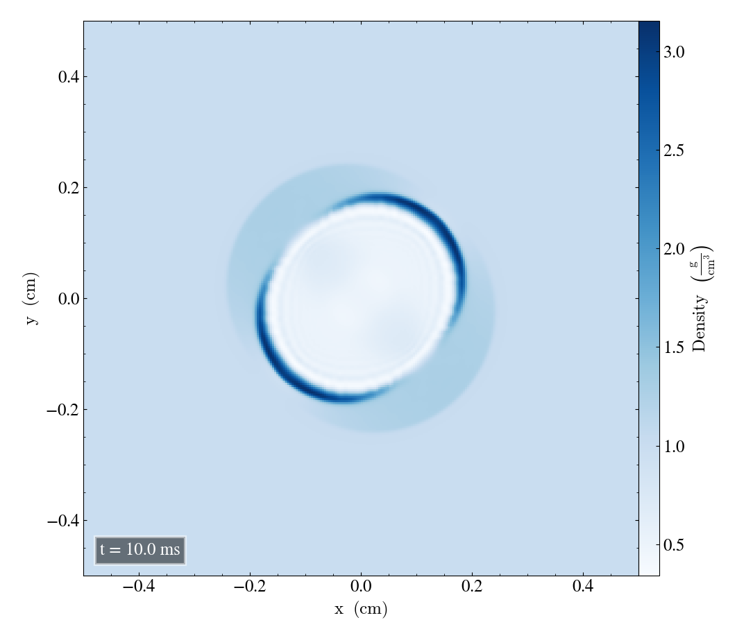
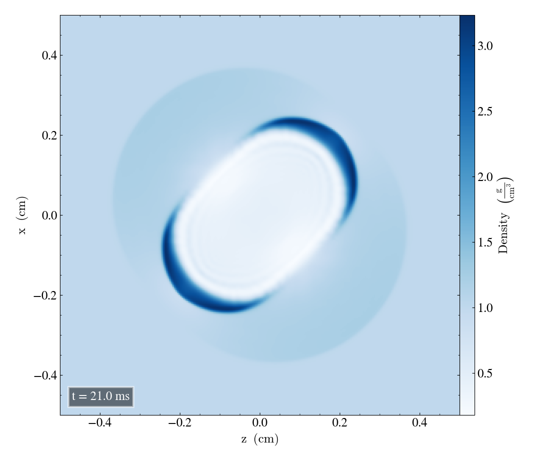
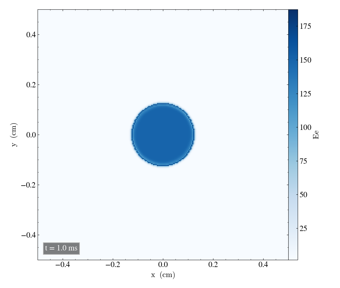
We will now plot the density, energy, velocity magnitude and magnetic pressure with the initial bifrost_params unadjusted. For the density, we will include plots in the xy-plane, xz-plane and yz-plane. For the remaining quantites, we will plot in the xy-plane only. In each plot, we will include a figure of the initial configuration at t=1ms and at t=21ms.
Densities
For the xy-plane we have
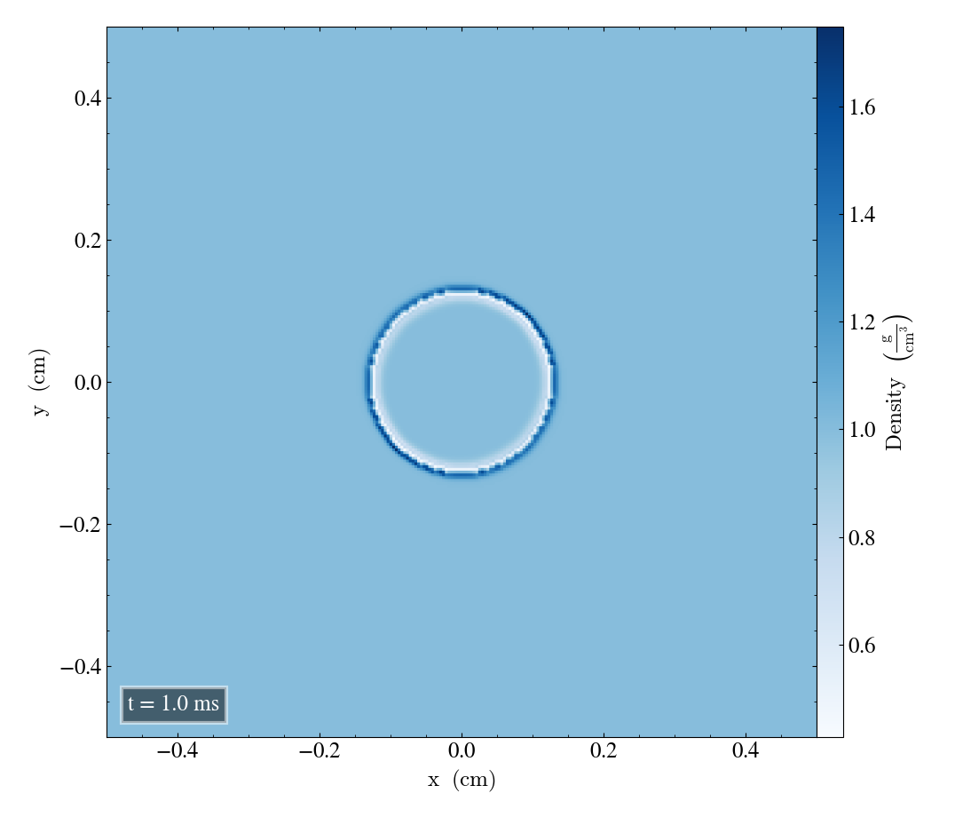

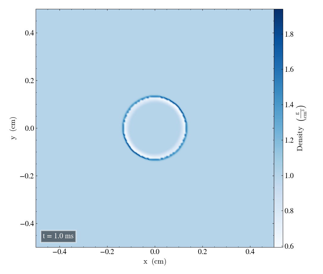
We also include an image of the density in the xy-plane after t=1.0ms to compare the evolution when we adjust the bifrost parameters, shown below.
For the xz-plane we get

Finally, for the yz-plane we get


Energy
The energy in the xy-plane looks like this

For the xz-plane we get

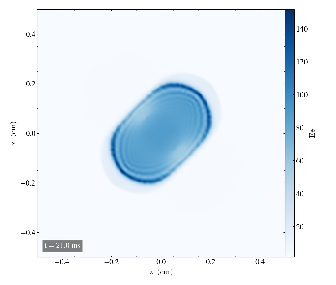
Finally, for the yz-plane we get


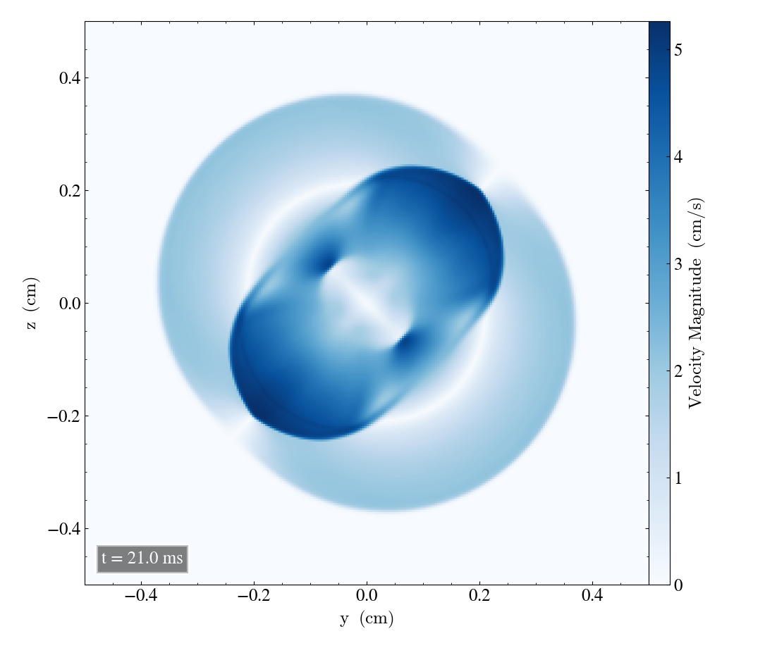
Velocity mangnitude
The velocity magntiude in the xy-plane becomes

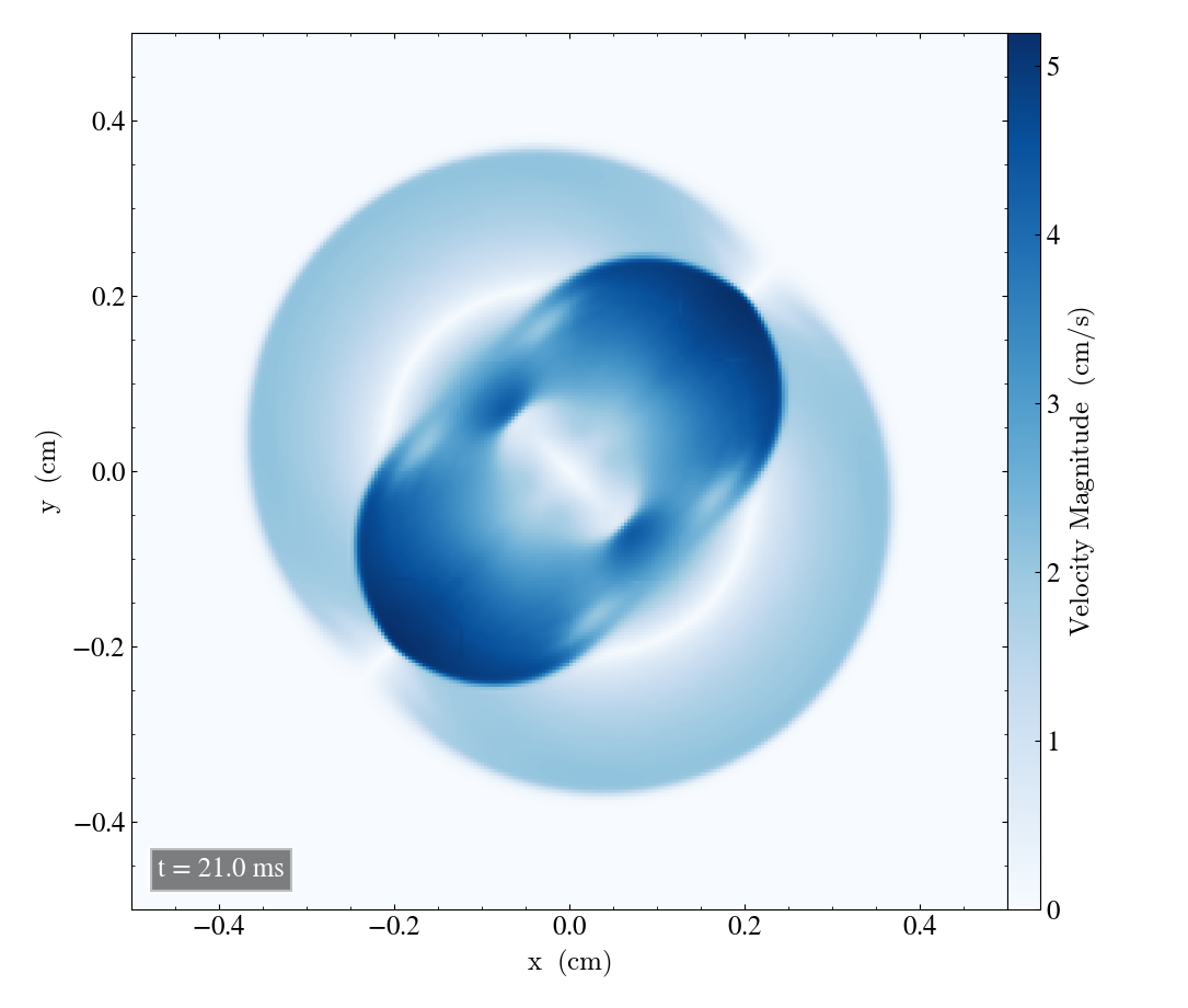
For the xz-plane we get
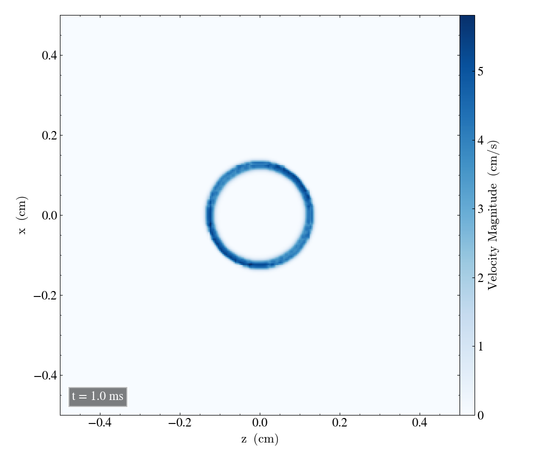

Finally, for the yz-plane we get


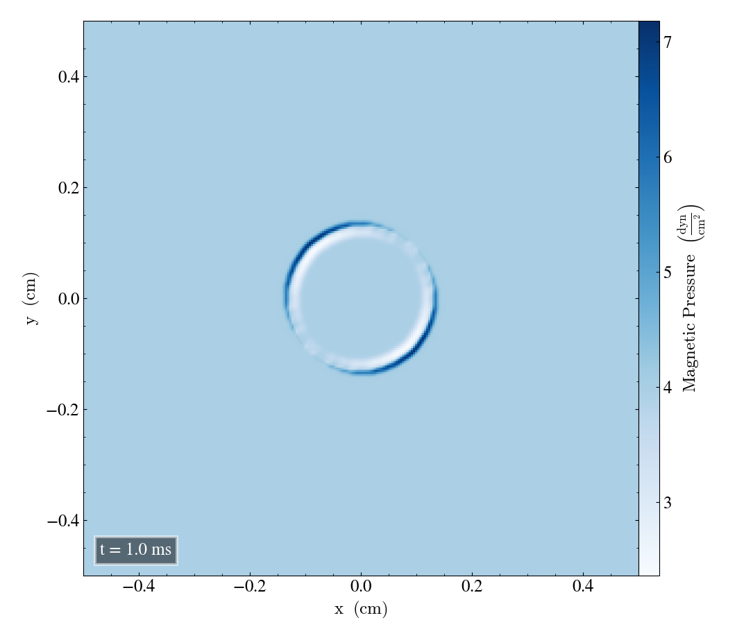
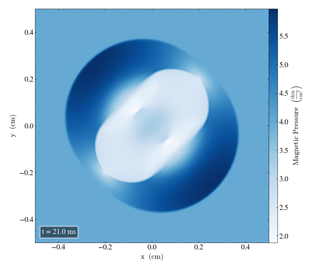
Magnetic pressure
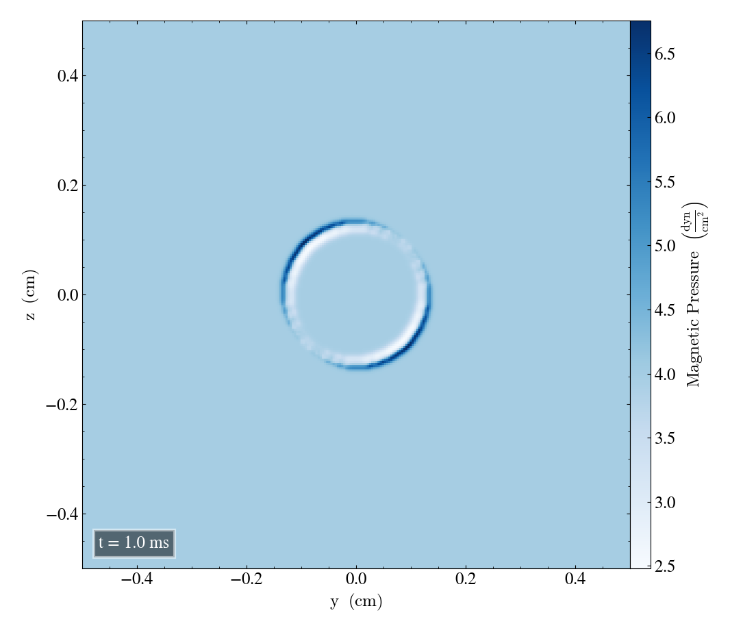
Finally, the magnetic pressure in the xy-plane is shown below.


For the xz-plane we get

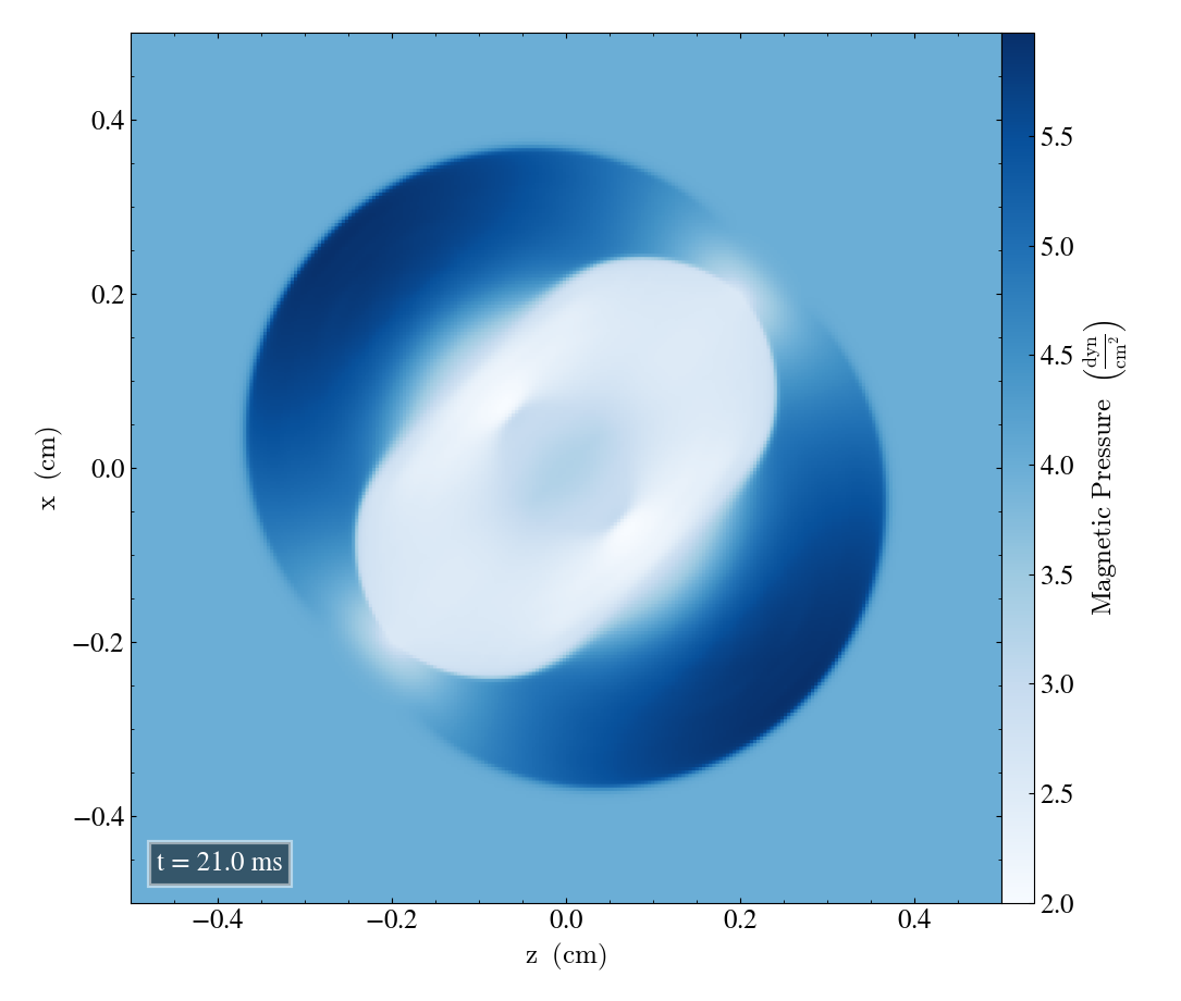
Finally, for the yz-plane we get

Increasing bifrost_params
Now, we will subsequently increase each bifrost_param while keeping all other parameters fixed. All parameters are increased be a factor 10, except from E=0.9, which was increased by a factor 5, since E=9 caused the simulation to crash towards the end. We start by plotting the density when each parameter has been changed.
Densities
We start by looking at the resulting densities
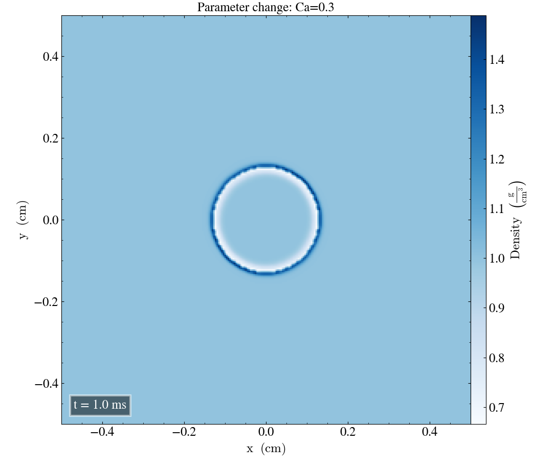
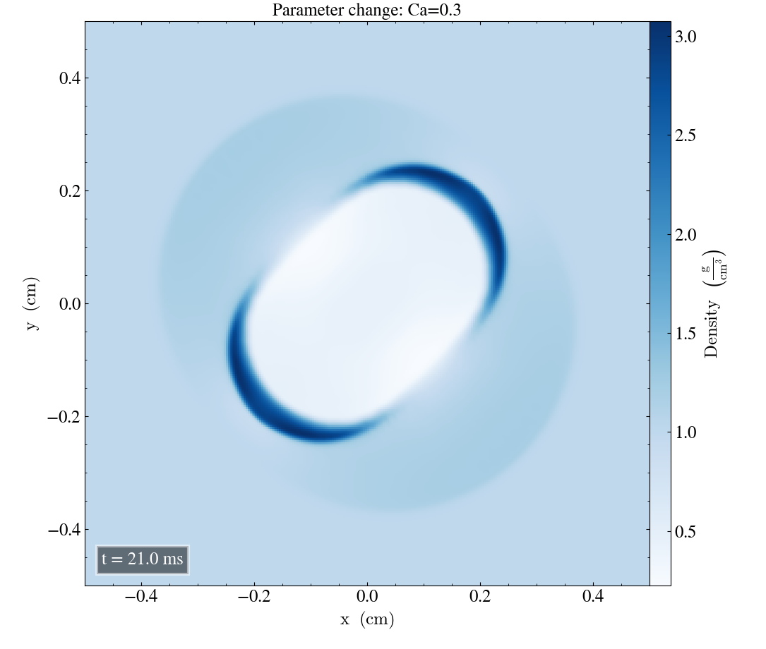
The above image with Ca adjusted yields a slightly reduced density magnitude at t=1ms. After 21ms the contours inside the white middle region is very dim, compared to the original plot.
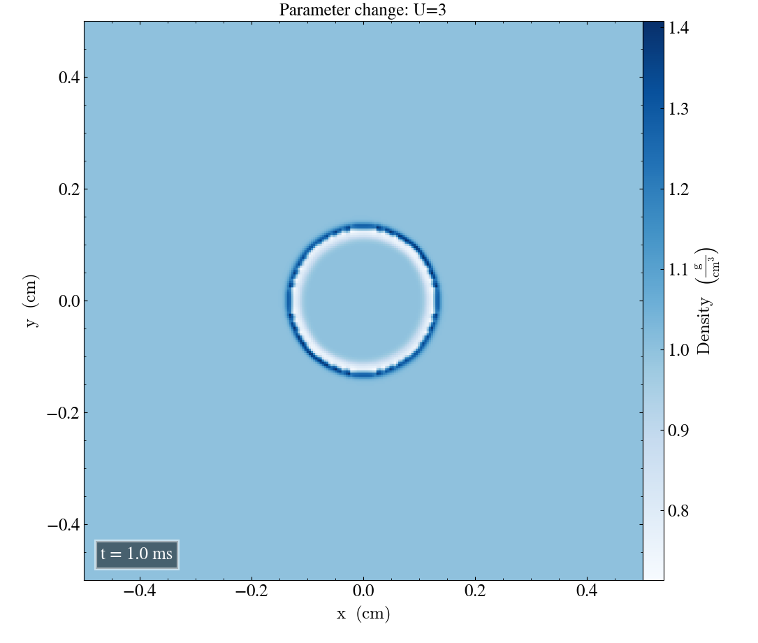
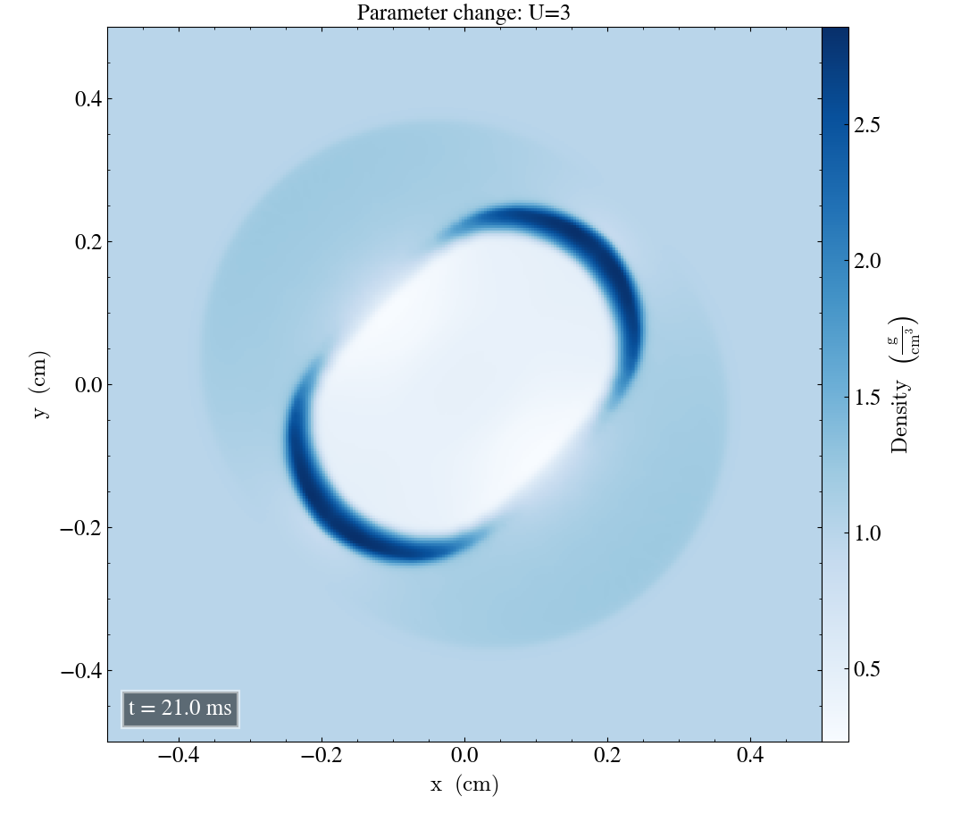
The above image shows a reduced density magnitude after t=1ms with U=3. The reduction is also present after t=21ms, and the contours are dim here as well.
For Uv=1, there was no visible changes to the result.

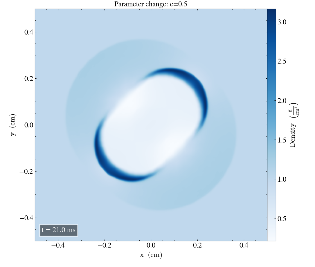
The above panel shows d=0.5 to the left and e=0.5 to the right, both after t=21ms. These parameters seem to affect the result in the same way, where the contours inside the white are barely visible. For d=0.5, there seems to be a slight deviation near the upper right and lower left corner, where there is a small reduction in density in the middle of the strongest region. None of the above parameters caused noticeable changes at t=1ms.
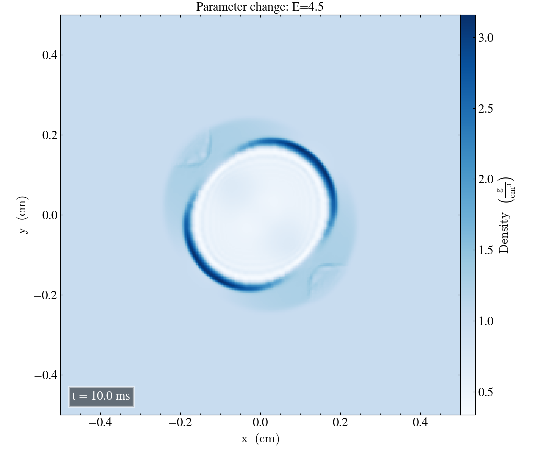
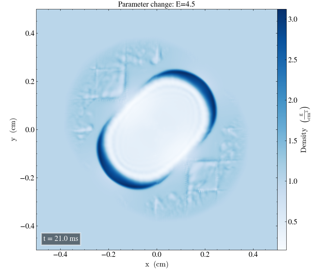
Finally, for E=4.5, there is no apparent change after t=1ms. After t=10ms, there is noticeable changes outside the blast contour. This is clearly visible after t=21ms.
Energy
Now, we plot the energy

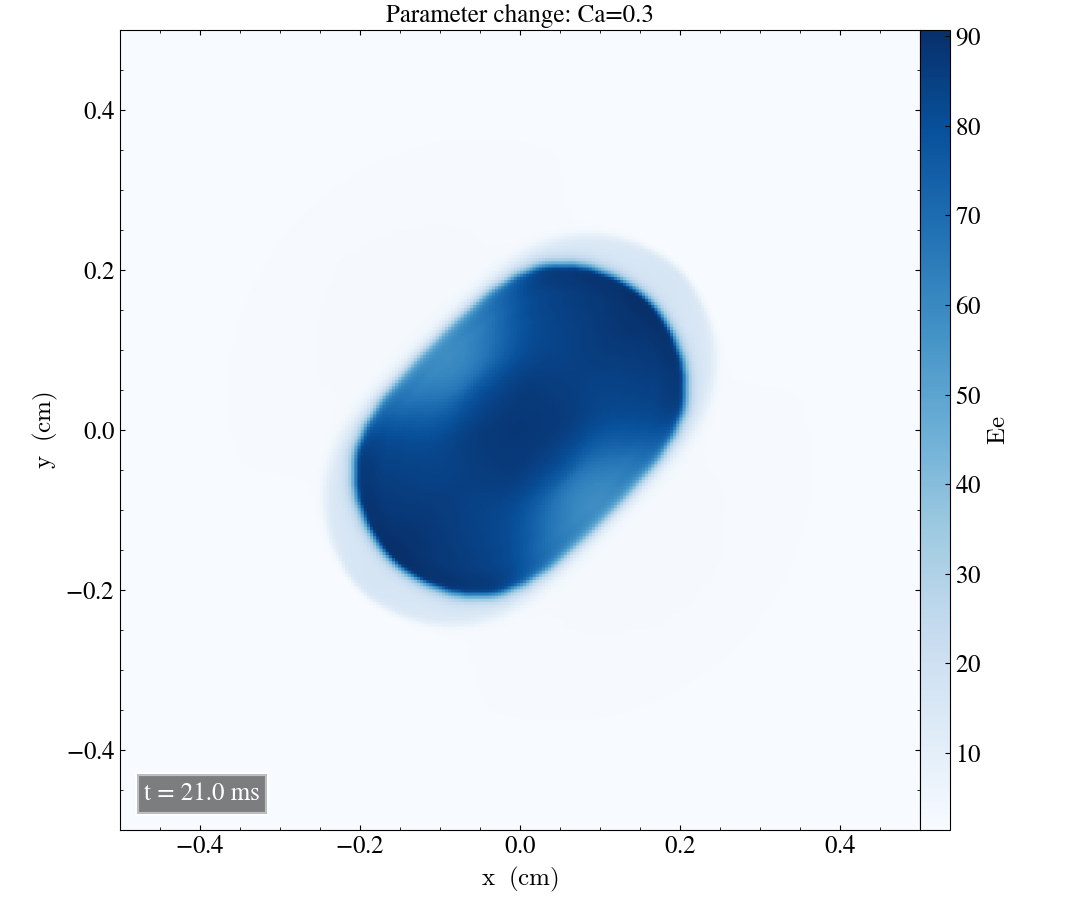
For Ca=0.3, there is a reduced maximum value of the energy. The initial plot seemed to have maximum energy on the outside edge of the blast region, while the above plot seems to have the energy maxima inside the edge. After t=21ms, the energy is clearly reduced, and the contour lines are no longer visible.

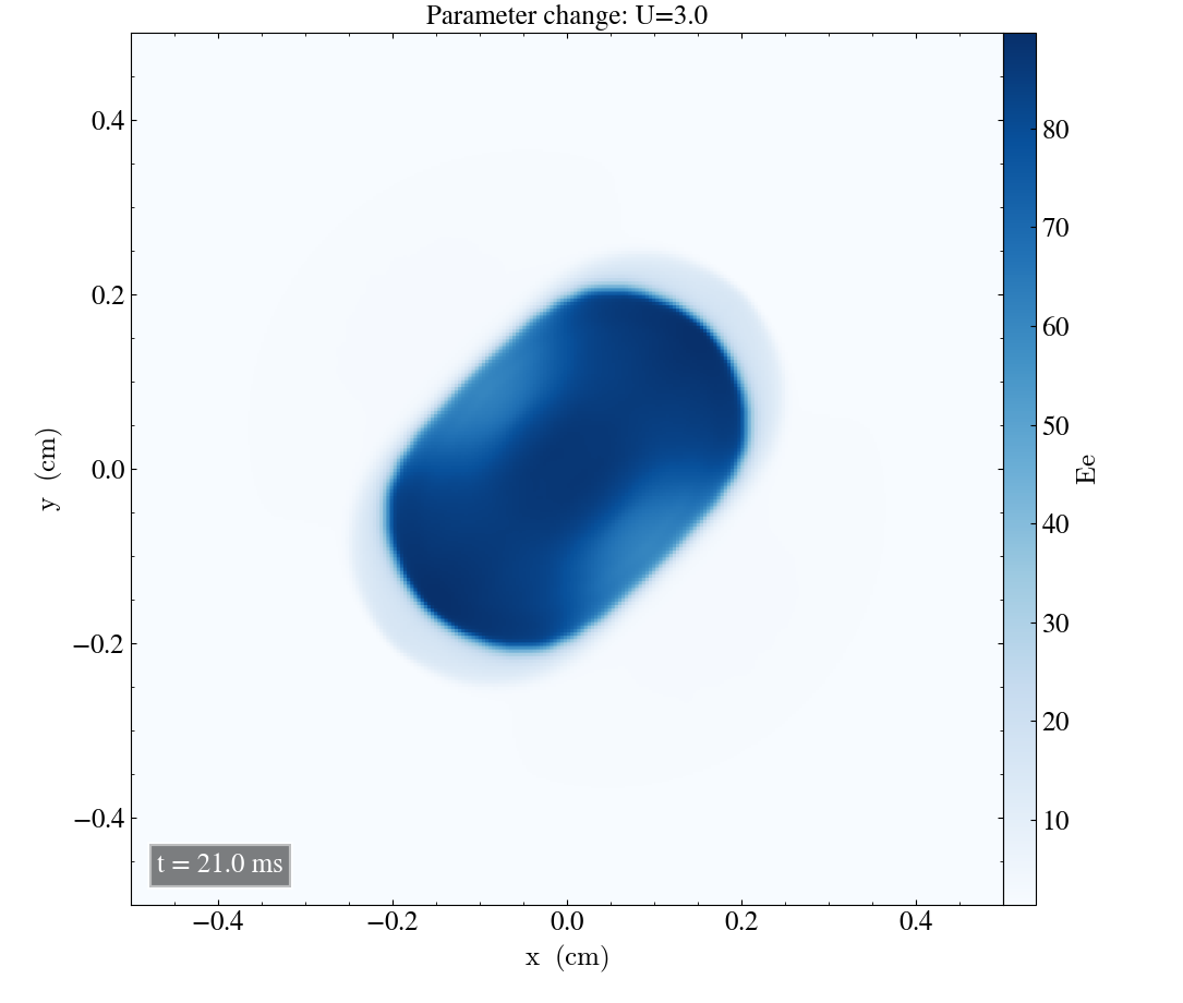
For U=3, the results are almost identical to the ones obtained by Ca=0.3, but with a slightly lower maximum energy value.
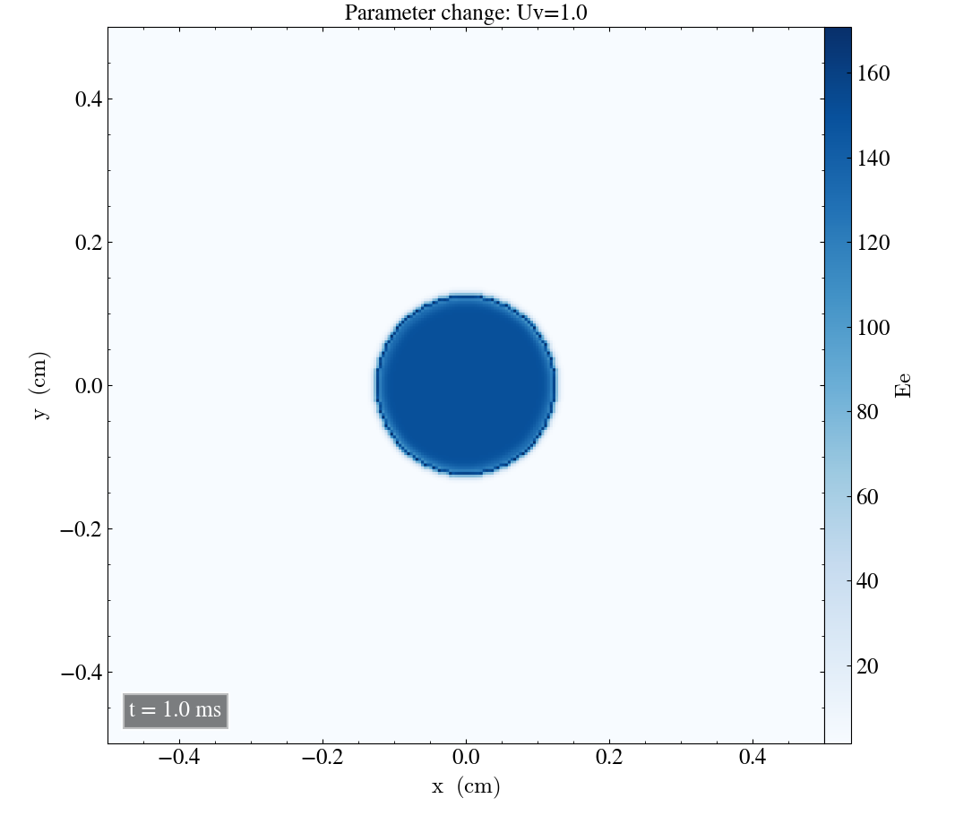
For Uv=1, there is a slight reduction in energy value after t=1ms, but after t=21ms it doesn’t visibly differ from the initial result.


Above, we see the results from d=0.5 and e=0.5. These seem to affect the result similarly to Ca=0.3 and U=3 respectively, with e=0.5 having a slightly lower maximum value than d=0.5 after t=21ms. We do however notice that d=0.5 has a thin edge on the outside after t=1ms, which is not present for e=0.5. This contour is also the behaviour we see in the initial simulation.
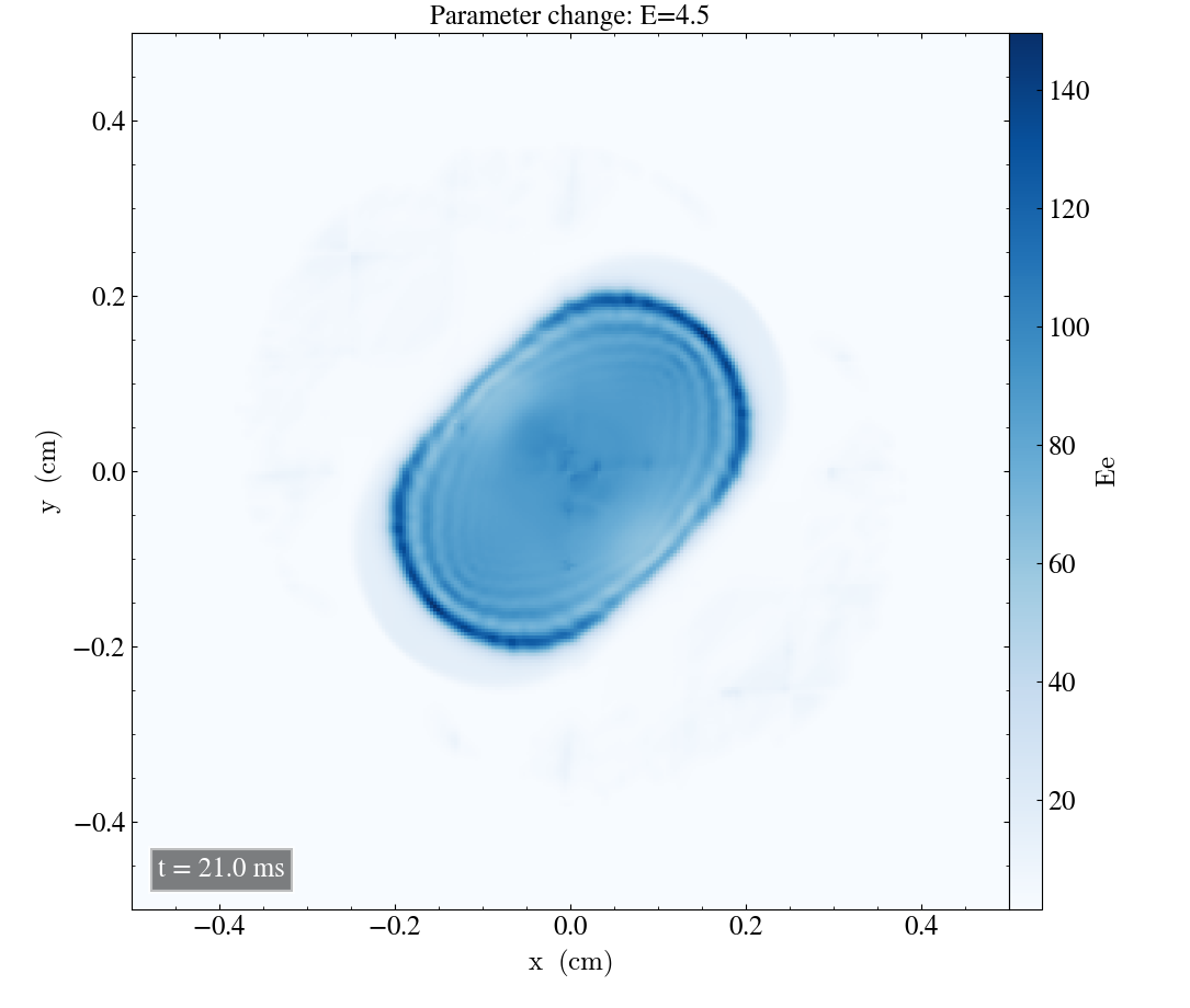
Above we see the result of E=4.5 after t=21ms. There were no visible deviation at t=1ms for this configuration. After t=21ms, there is some noisy features inside the center, and there is also strange behaviour on the outside, somewhat similar to what we saw for the density plot.
Velocity magnitude
Now, we plot the velocity magnitude

With Ca=0.3, the only noticeable difference is a reduced magnitude after t=1ms, shown above.

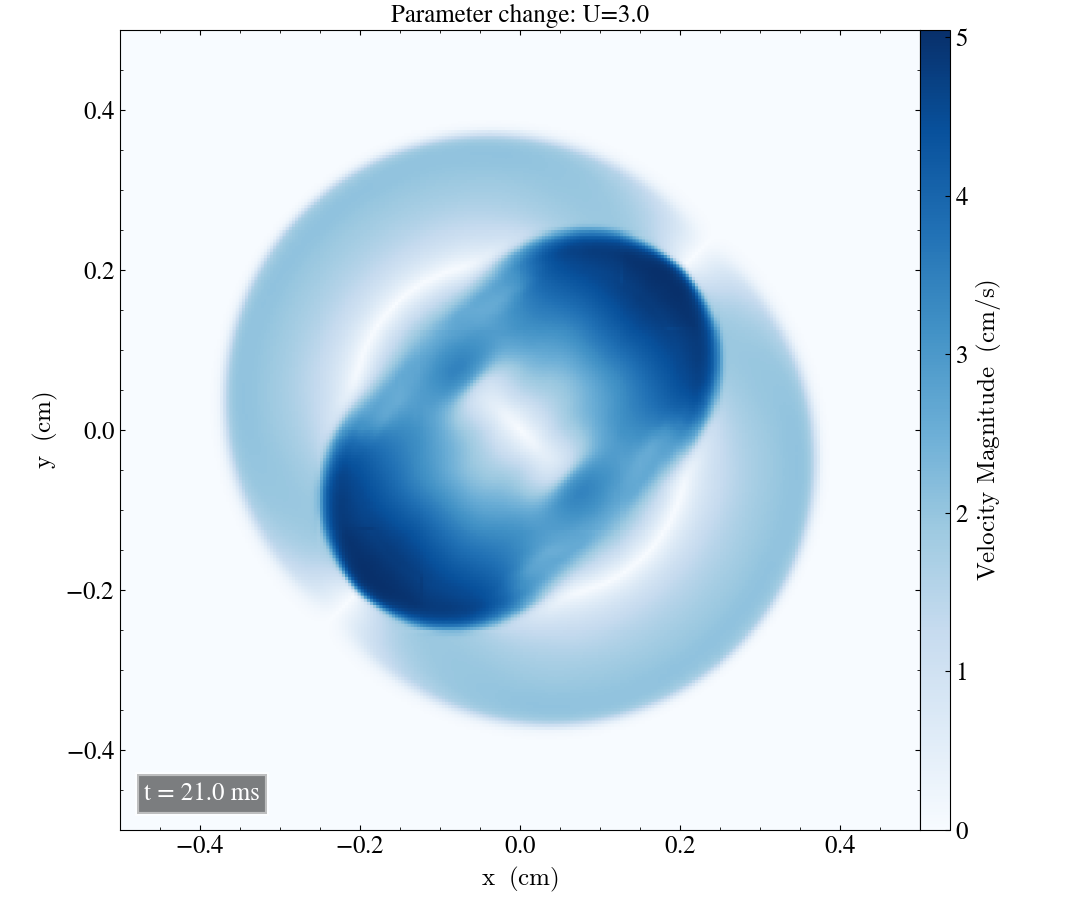
For U=3, there is a further reduced velocity magnitude after t=1ms, and after t=21ms, the resulting plot seems to be smeared out. The edges and contours are less clear and the details are less apparent overall.
The case with Uv=1 yielded no noticeable changes.
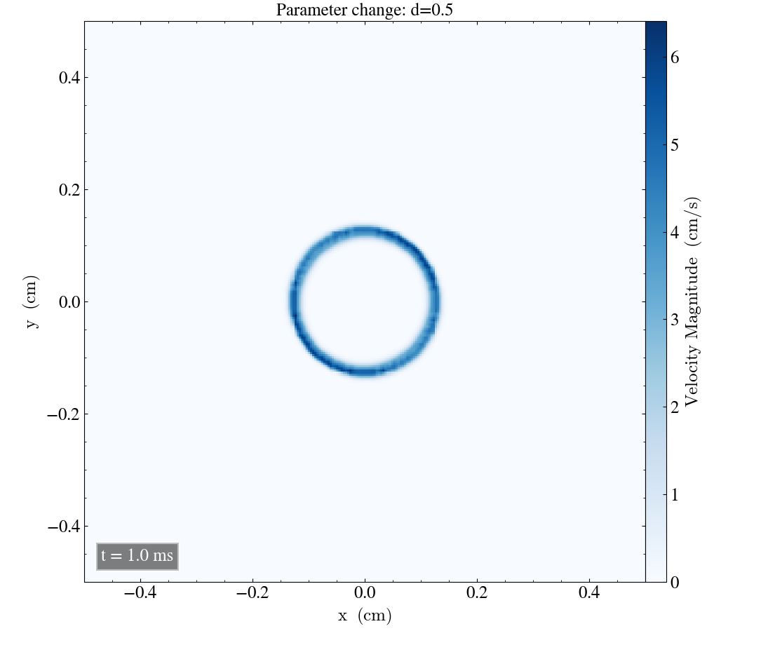
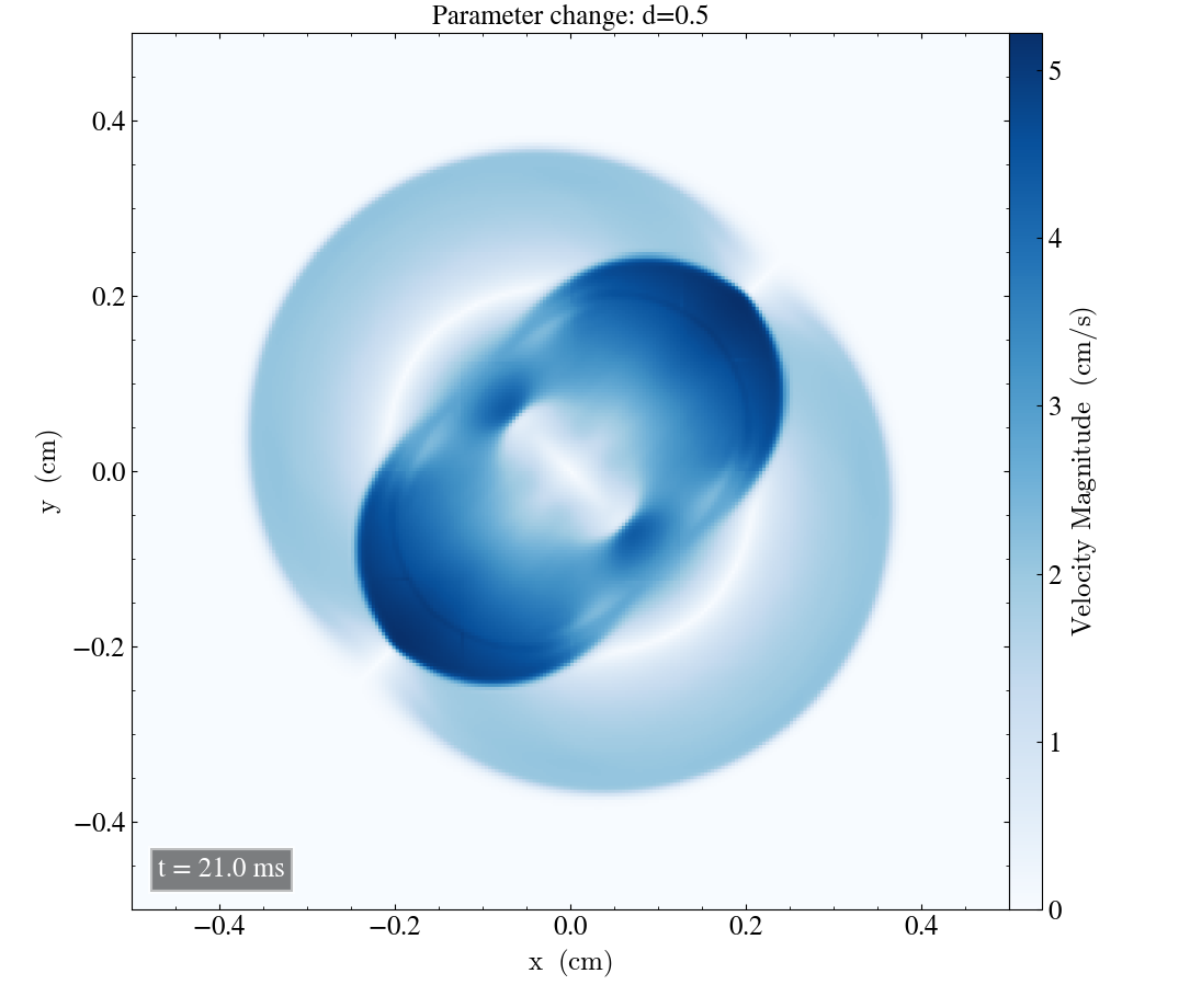
for d=0.5, the velocity magnitude has a higher maximum after t=1ms. After t=21ms, there is a dark line near the edges of the elliptic profile.
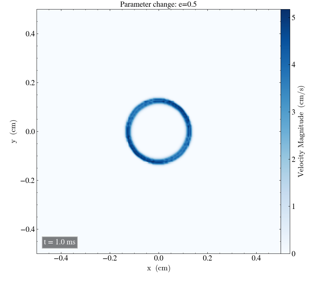
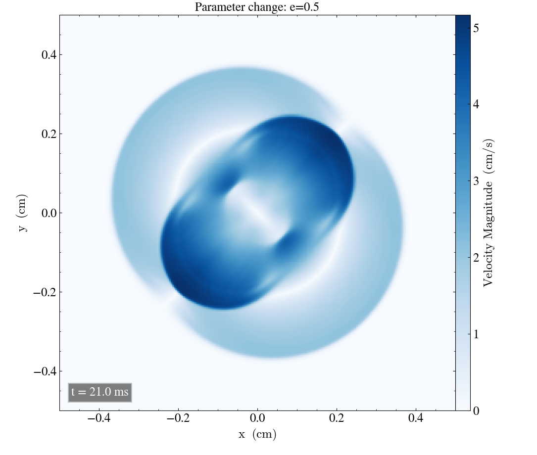
For e=0.5 there is a reduced maximum velcity magnitude after t=1ms. After 21ms, there is a line inside the elliptic shape, with the same shape as we got from d=0.5, but this is lighter. For d=0.5 there was a velocity increase at this region, but e=0.5 yields a velocity decrease.
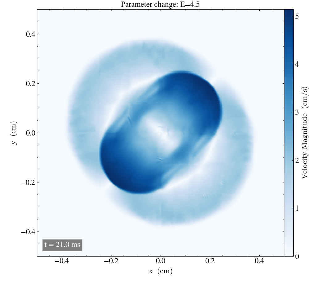
After t=1ms, there is no noticeable difference with E=4.5. After t=21ms, the above plot shows noisy behaviour throughout the entire region where velocities are nonzero.
Magnetic pressure
Now, we plot the magnetic pressure
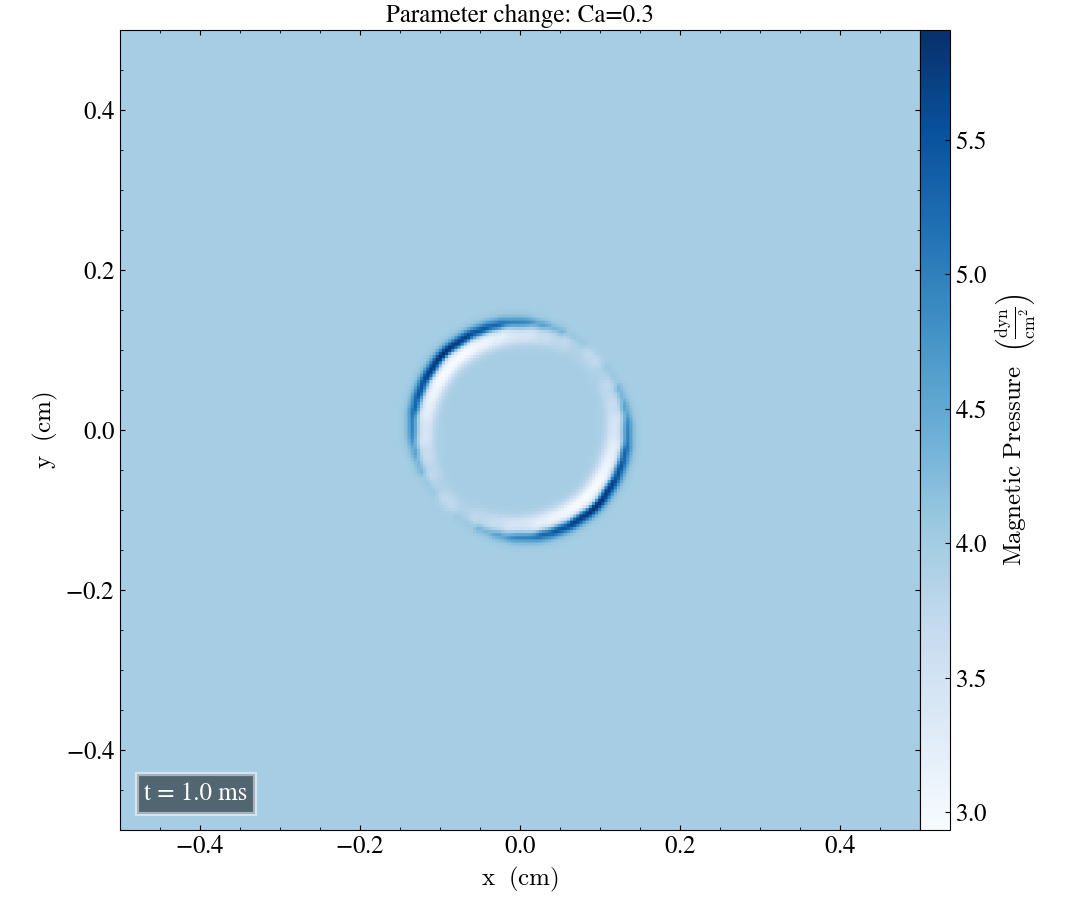

At t=1ms, Ca=0.3 and U=3 yields a decreased maximum value of the magnetic pressure, shown in the left and right pnale above, respectively. Neither parameter caused noticeable differences after t=21ms.
Uv=1 did not visibly affect the magnetic pressure within t=21ms. Neither did d=0.5 or e=0.5.
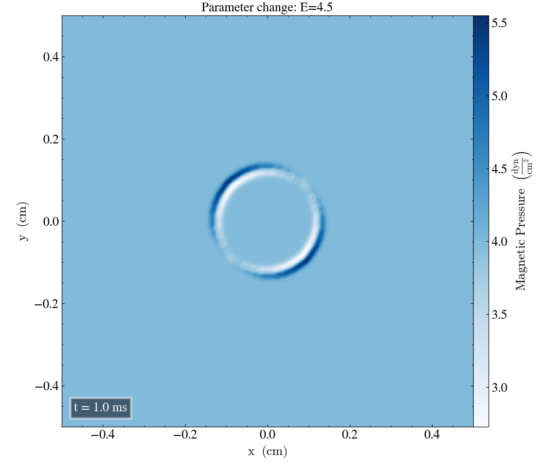
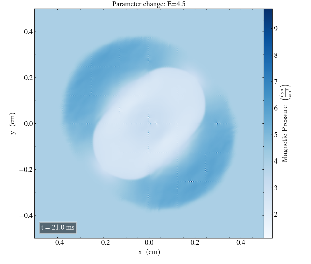
With E=4.5, we see a reduced maximum value of magnetic pressure after t=1ms. After t=21ms, there is a lot of noise once again for this parameter. It seems to be very dim, but the maximum value at the colorbar is above 9 (compared to ~5.5 iriginally), which is caused by small dots around the plot with apparently large values. These dots seem to be aligned on an 8x8 grid in the plot, which coincides with the size of the computational box, which is (x,y,z)=(8,8,1) for this simulation.
Ramses/mhd_eos
- Now we run the experiment with the solver ramses/mhd_eos. The initial simulations were run with the same configurations as we used for the bifrost solver, and we use the ramses_params
slope_type=3.5
Initial results
We will now plot the resulting density, energy, velocity magnitude and magnetic pressure in the xy-plane, xz-plane and yz-plane for the ramses solver. We plot the initial result at t=1ms, and at the final time of t=21ms.
Densities
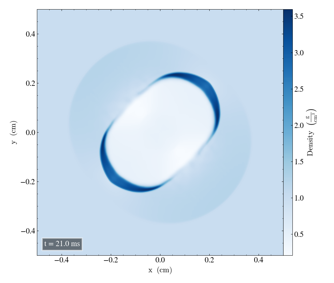
Below, we plot the initial and final densities. We begin with the xy-plane, shown below.
Below, shows the xz-plane


Finally, the yz-plane


Energy
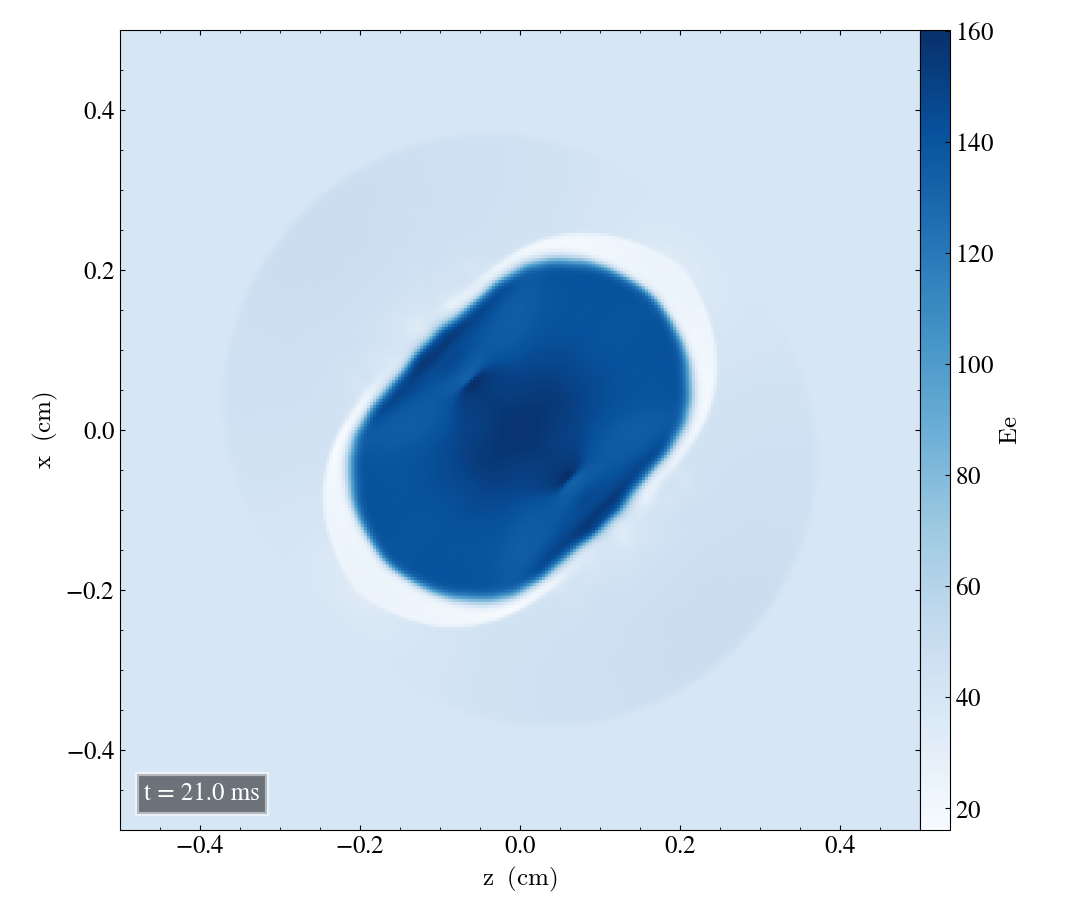
We now plot the energy, starting with the xy-plane, shown below


Then we plot in the xz-plane

Finally, the yz-plane


Velocity magnitude
We begin with the xy-plane, shown below


We continue with the xz-plane


Finally, the yz-plane

Magnetic Pressure
Finally, we look at the magnetic pressure, starting with the xy-plane, shown below
We continue with the xz-plane


Finally, we plot the yz-plane


Testing different slope types
Now, we will adjust the slopes to see the resulting behaviour. The above plots were created using slope_type=3.5. The below studies shows the result of testing with slope_type values of 3, 2, 1 and -1.
Density
We start by looking at the density.
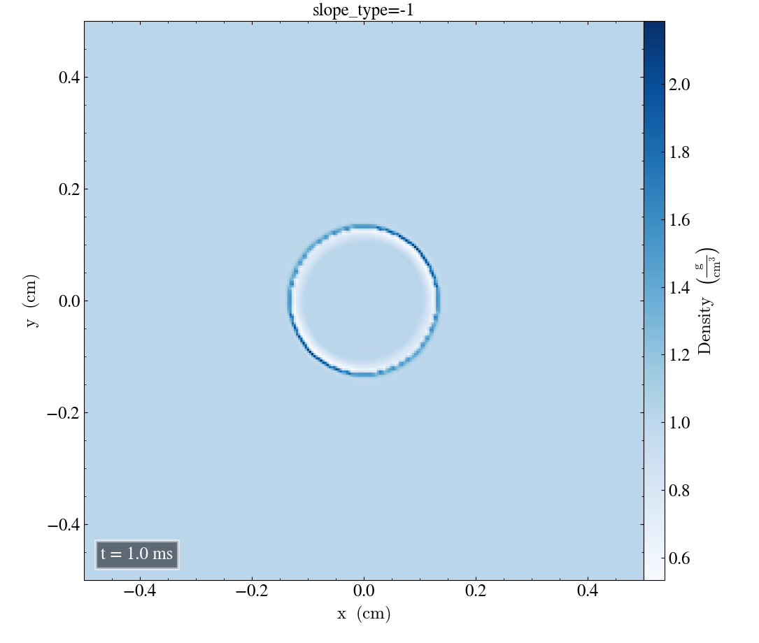
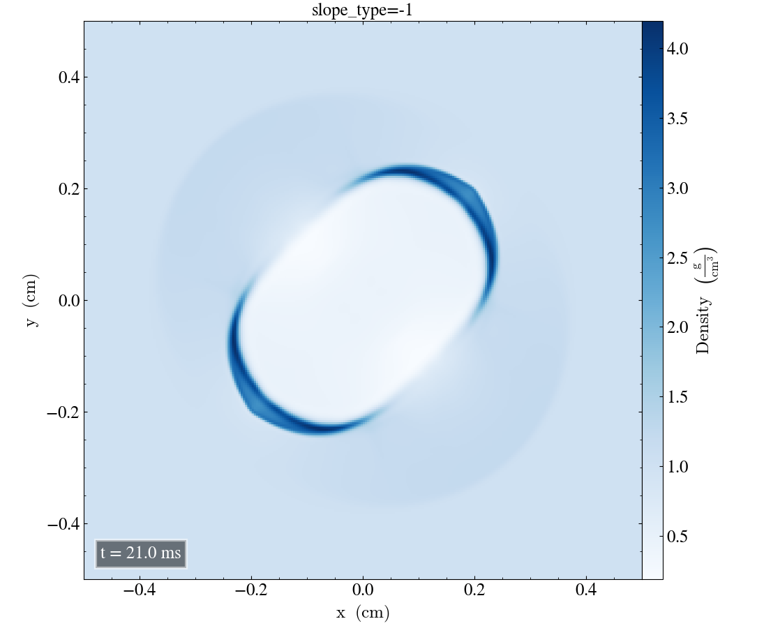
The above image shows the result of slope_type=-1. The density has an increased maximum value at both t=1ms and t=21ms. At t=21ms the elliptic profile is also more pointy near the edges.
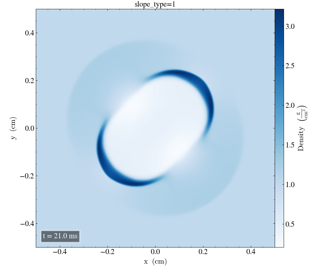
For slope_type=1, shown above, there was no visible change at t=1ms. After t=21ms however, there is a reduced density magnitude.
The results from slope_type=2 yielded no significant deviations for the density. The only difference was a slight increase in the maximum density values at both t=1ms and t=21ms by a value of less than 0.1. Other than that, there were no visible changes.
For slope_type=3, there was a slight decrease in maximum density value of both t=1ms and t=21ms. The decrease at t=1ms was around 0.1 g/cm3, while the decrease at t=21ms was between 0.3-0.4 g/cm3.
Energy
We will now study how the energy is affected by the different slope_type values.
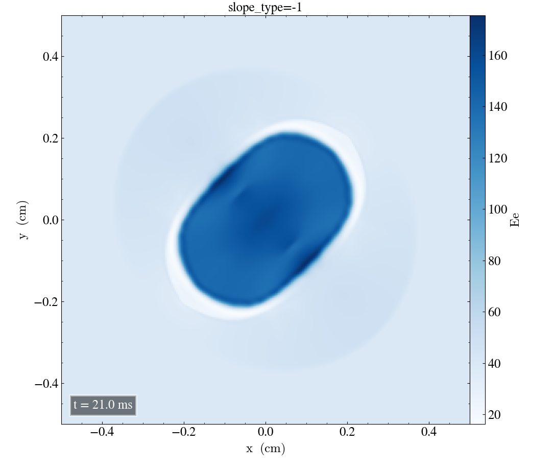
Above swows the result of slope_type=-1 after t=21ms. For t=1ms, there was no apparent change. After t=21ms, there is a slight increase in the maximum energy values, and energy in the center seems more evenly distributed with less details. This may be due to the increased maximum value.
With slope_type=1 and slope_type=2 there were no apparent changes in the resulting energy after t=1ms or t=21ms.
With slope_type=3 there was no change after t=1ms, and after t=21ms, there was only a minor reduction in the maximum density value, barely visible from the colorbar.
Velocity magnitude
We will now study the velocity magnitude with different slope_type values.
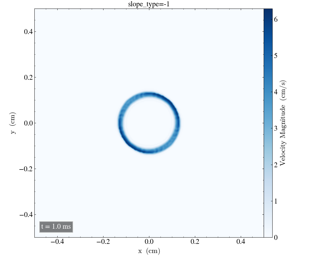
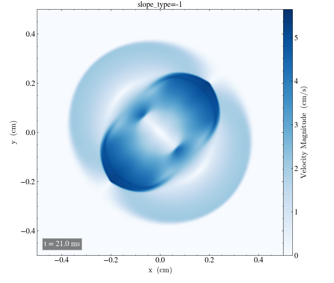
With slope_type=-1, shown above, the only noticeable change is a minor increase in velocity magnitude after t=1ms and a slightly larger increase after t=21ms. Otherwise, there is little change.
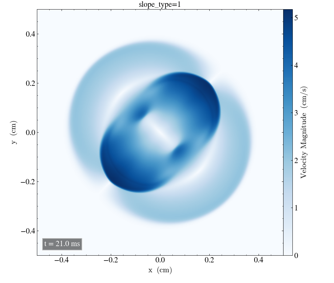
After t=1ms, slope_type=1 yielded a minor reduction in the maximum value of the velocity magnitude after t=1ms, which was barely visible. After t=21ms, the colors inside the elliptic shape is darger, and lacks many of the details that were present in the initial case.
With slope_type=2 and slope_type=3, the only change visible was a slight reduction in maximum magnitude at t=1ms for the latter case.
Magnetic pressure
Finally, we are going to study the magnetic pressure results.


With slope_type=-1, shown above, the maximum pressure value is lower after t=1ms. After t=21ms, the elliptic contour near the center is more stretched out towards a circle. In the initial plot, there seemed to be straight lines from the bottom left to the top right which separated the regions with high and low pressure values. These lines do no longer appear straight in the above image.

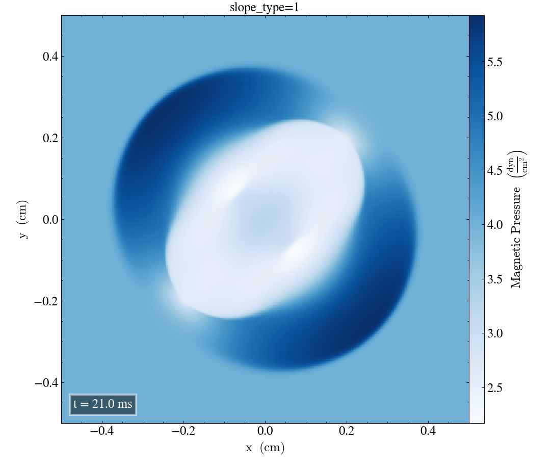
With slope_type=1, as shown above, there is a further reduction of the initial pressure values at t=1ms. After t=21ms, we see the same effect as we did with slope_type=-1, namely a rounding of the elliptic shape in the center.
Slope_type=2 resulted in no visible changes after t=1ms or t=21ms.

With slope_type=3, there was a slight reduction in maximum magnetic pressure value at t=1ms, shown above. After t=21ms, there were no changes clearly evident.