Magnetic Field Loop Advection
In this experiment we report the results of the Magnetic loop advection experiment, where we study the result from changing different bifrost parameters for the bifrost solver and slope_types for the ramses/mhd_eos solver.
- The experiment was run on
branch: develop
hash: aff3841
Simulation parameters
We will here report the initial parameters used for running the experiment. We tabulate the grid parameters for the xy-direction explicitly, and state the differences related to the other planes
Output parameters
For the output parameters
out_params |
||
|---|---|---|
end_time |
out_time |
print_time |
2 |
0.2 |
0 |
Using end_time=2.0, the magnetic loop completes two whole cycles for the initial velocities and cartesian parameters we have used, which is stated below.
Initial conditions
For the xy-plane we have
cartesian_params |
||||
|---|---|---|---|---|
size |
dims |
mpi_dims |
origin |
periodic |
2,1,0.0625 |
4,4,1 |
1,1,1 |
-1,-0.5,0 |
t,t,t |
patch_params |
||||
|---|---|---|---|---|
nt |
n |
no_mans_land |
do_check_nan |
grace |
5 |
32,16,1 |
t |
t |
0.05 |
IC_params |
||
|---|---|---|
idirect |
ux |
uy |
3 |
2 |
1 |
Where ux=2 and uy=1 causes the loop to move from it’s initial position at the box’s center and towards the upper right corner.
For the zx-plane the simulation was run by using n=16,1,32, and changing the other parameters accoridnagly. For the yz-plane the simulation was run by setting n=1,32,16, with the remaining parameters changed accoridngly. For the yz-plane idirect=1 and for the zx-plane idirect=2.
Solver parameters
- For the gas, we used a gamma-law equation of state with
gamma=5/3
Bifrost parameters
For the bifrost solver we initially used
bifrost_params |
|||||
|---|---|---|---|---|---|
Ca |
U |
Uv |
d |
e |
E |
0.05 |
0.1 |
0.2 |
0.05 |
0.05 |
0.5 |
Ramses parameters
- For the ramses solver, we initially used
slope_type=3.5
Initial results with unchanged parameters
We will here report the initial results where we use the bifrost parameters listed above. Initially, we plot the result after t=0s and t=2s for all three planes, in order to check for differences.
For the xy-plane we get


For the zx-plane we get

And finally, for the yz-plane


Behaviour of loop in the xy-plane
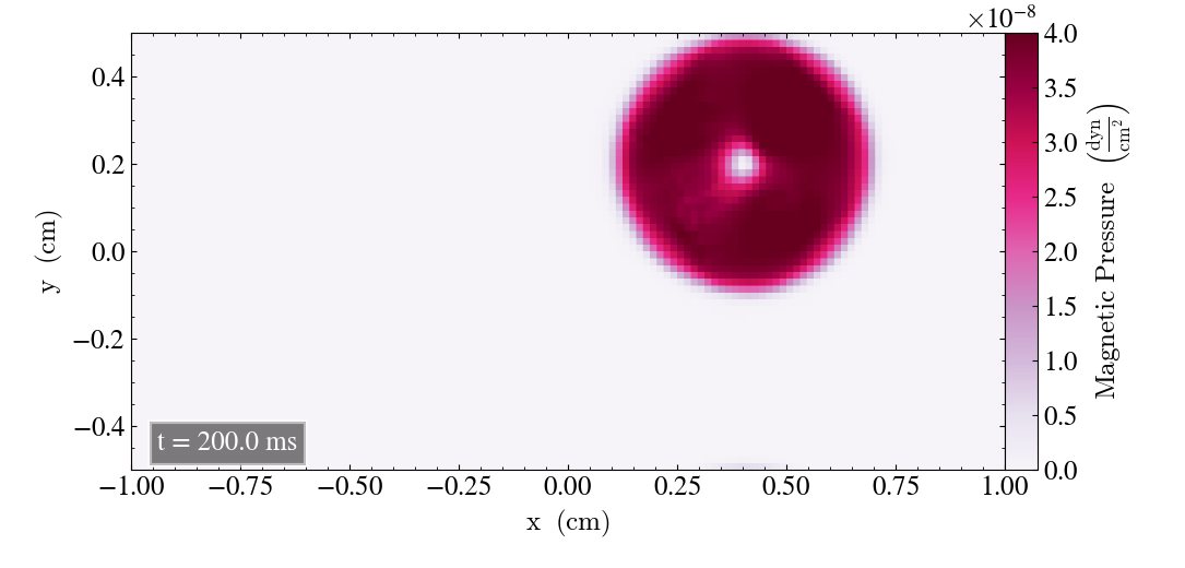
Now, we include snapshots of the run in the xy-plane to show the behaviour of the loop throughout the simulation. This will be used for comparison later on. The image after t=0s is omitted, as it is shown above.
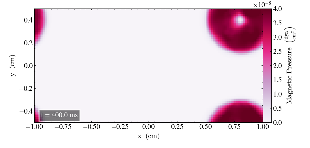
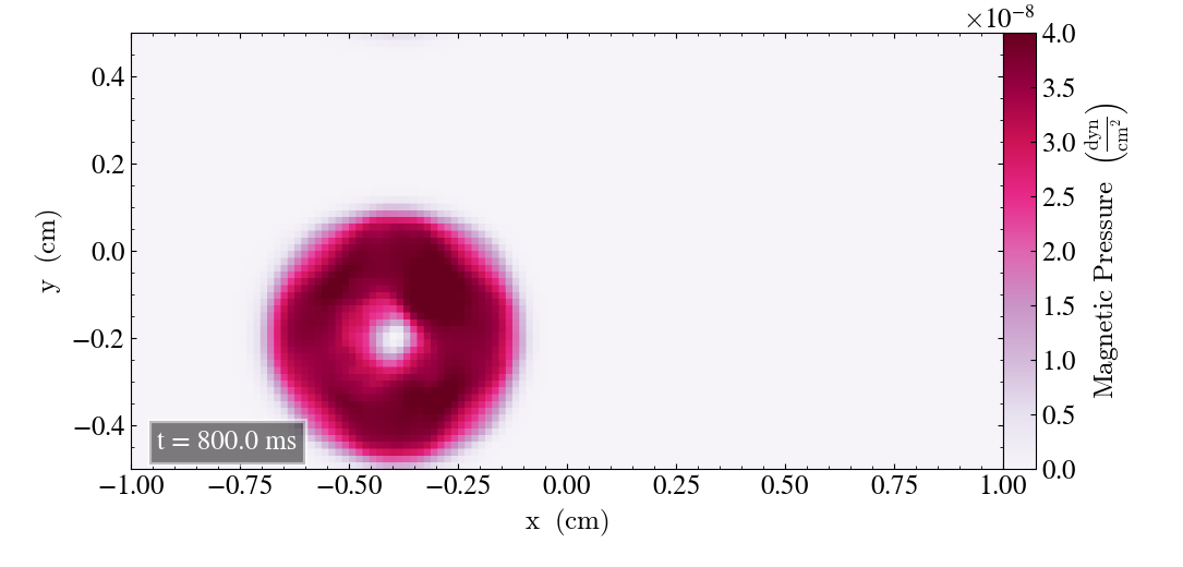
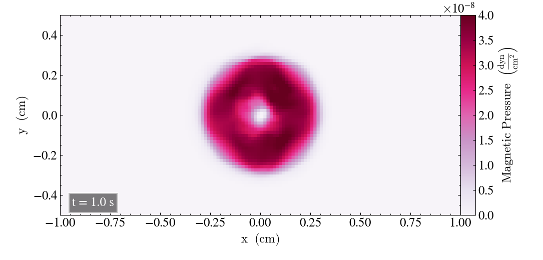
And the loop has returned to the initial state after t=1s.
It continues for an additional cycle after t=1s. Below shows the simulation after t=1.2s and t=2s in the left and right panel, respectively, where the simulation ends after t=2s.
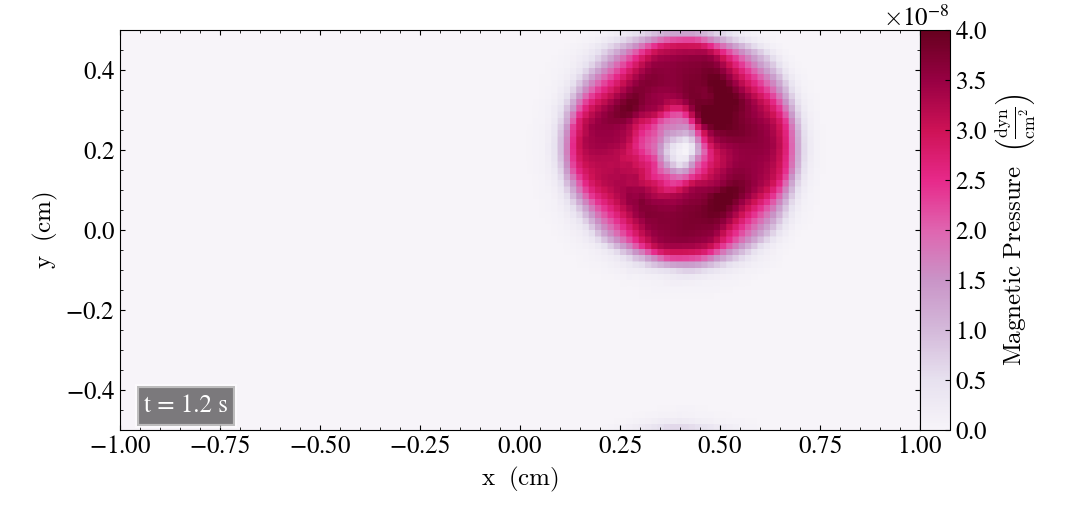
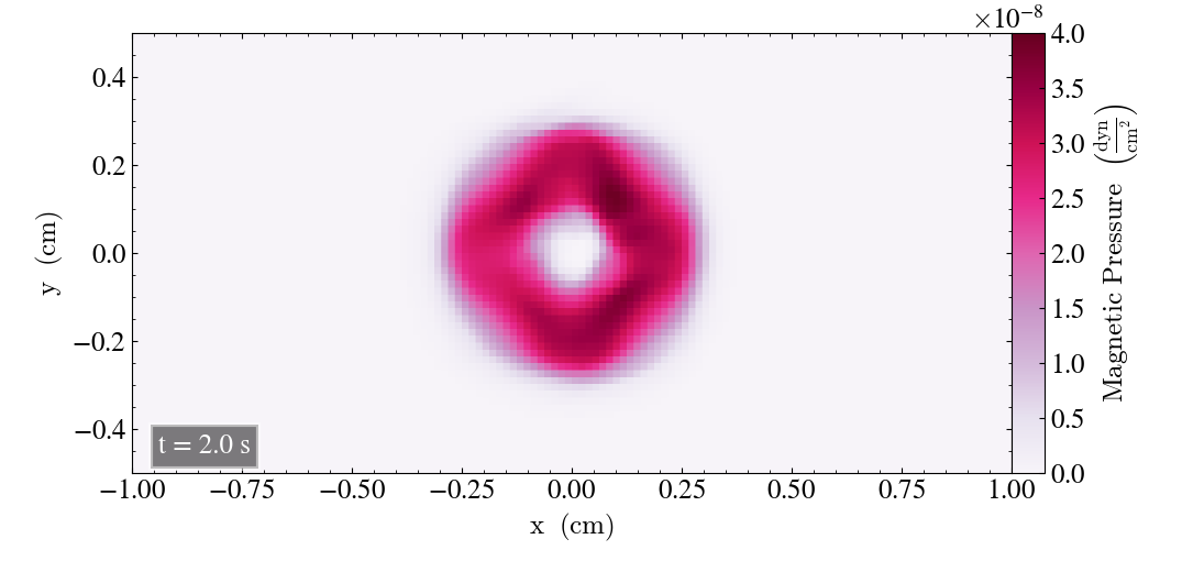
We see that the final image has a larger pressure drop at the center and a lower pressure magnitude overall.
Static behaviour
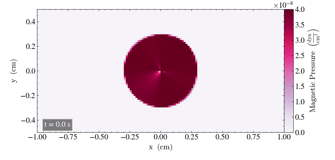
We will now check the behaviour of the loop for the static case, where we set the u-values (ux, uy, uz) to zero for all the directions. We will plot the result for t=0s and t=2s for all three directions.
For the xy-plane we get

For the zx-plane we get

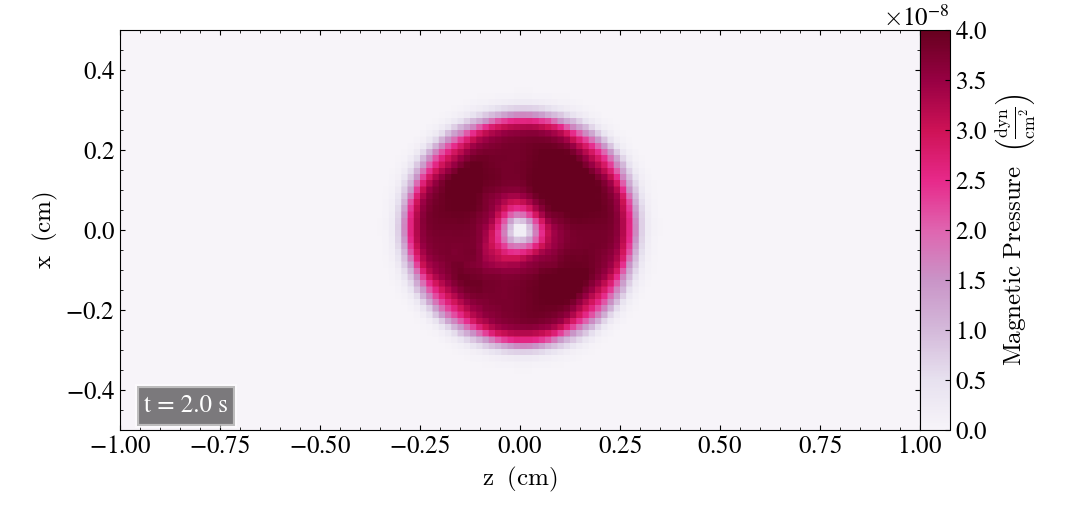
Finally, for the yz-plane we get


For all three planes, the static Loop yields a lower reduction in magnetic pressure throughout the simulation, and that the Loop is less deformed compared to the moving Loop, as it has a more circular shape. The hole in the center of the Loop has a size comparable to the hole of the moving loop after t=1s.
Normalized magnetic pressure evolution
We will now study the evolution of the normalized magnetic pressure throughout the simulation.
Increasing and decreasing bifrost parameters
We begin by studying the effect of subsequently increasing each bifrost parameter while the other are held fixed. For the increase, all bifrost parameters were multiplied by a factor of 5, except from E, which was multiplied by a factor of 2.5 since E=2.5 caused the simulation to crash. The resulting normalized pressure evolution is plotted below on the left panel. On the right panel we show the effect of decreasing the bifrost parameters subsequently by a factor of 2, i.e. using half of the original values.
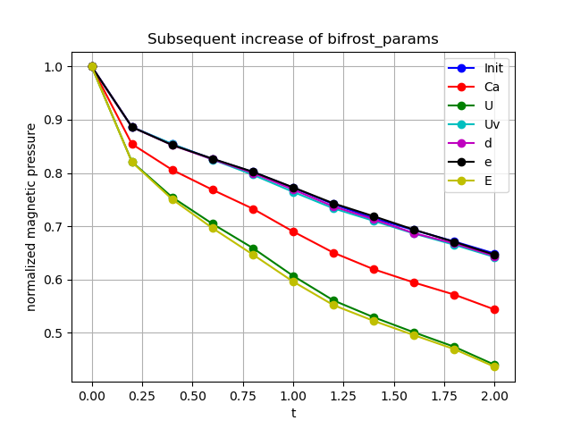
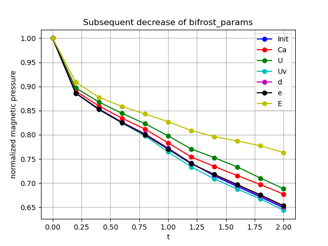
We see that there is little increase of the pressure by increasing the bifrost parameters. However, between t=1 and t=1.75 the pressure is higher than the initial value when the parameter e was increased to a value of e=0.25. The parameters Ca, U & E caused a significant pressure drop when increased. With decreased parameter there is a noticeable pressure increase when the parameters Ca, U & E were reduced, which are the same parameters that caused a pressure drop when increased. The parameter Uv causes the pressure to drop slightly when increased, while there is little noticeable change when the parameters d & e are reduced.
Comparing the above result with the ones obtained by Miniati & Martin (2011) the pressure decrease we see are far greater than the ones they obtained with the resolution N=128 in the x-direction, which we also used. After t=2s Miniati & Martin reports a normalized pressure value of more than 0.95. We compare this to the results from Gardiner & Stone (2005), where the magnetic pressure dropped from 3.46e-8 at t=0s to 3.18e-8 after t=2s, corresponding to a normalized final value of 0.91. These results were obtained with N=128 in the x-direction as well.
Further deacrease of bifrost parameters
Now, we report the effects by a further decrease of the parameters, where each parameter is subsequently reduced by a factor of 5 and by a factor of 10, shown in the left an right panel below, respectively.
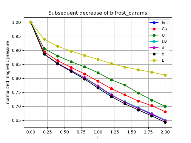
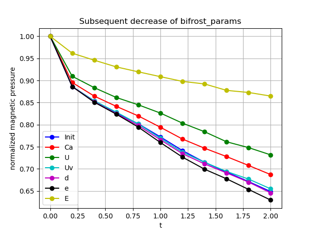
The image on the left panel below shows that Ca, U & E yields a higher pressure evolution than before. However, despite lying below the initial value when reduced by a factor 2, Uv lies slightly above the initial value when reduced by a factor of 5. This factor causes the pressure to lie below the initial one when adjusting e. On the right panel above we once again see the further increase in pressure for Ca, U & E. Uv lies below the initial result at first, but lies above towards the end of the simulation. e is clearly below the initial pressure result, while d now lies slightly below the initial.
With the reduction factor of 10, the E parameter adjustment yields a final normalized magnetic pressure value above 0.85. This is slightly higher than what Miniati & Martin achieved using N=32, while we use N=128. These are still below 0.91 which was achieved by Gardiner & Stone (2005).
There were few noticeable changes in the evolution of the Loop for the parameters that increased the pressure over time. However, the parameter E affected the behaviour of the magnetic pressure Loop once it became small enough. Below, we show images of the Loop after t=0.2s and t=2s when E is reduced. We start with the plot where it was reduced by a factor of 2, shown below.
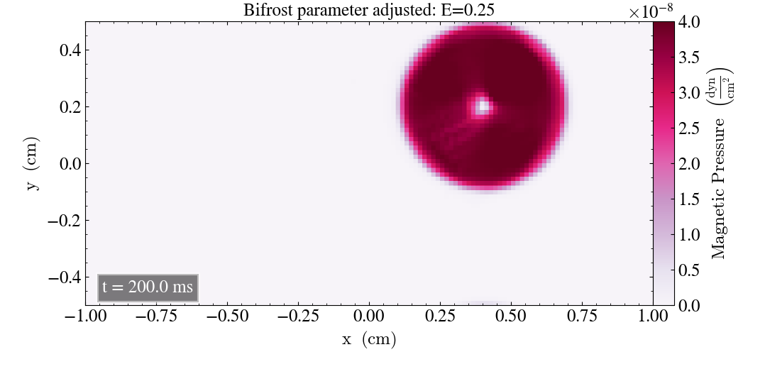
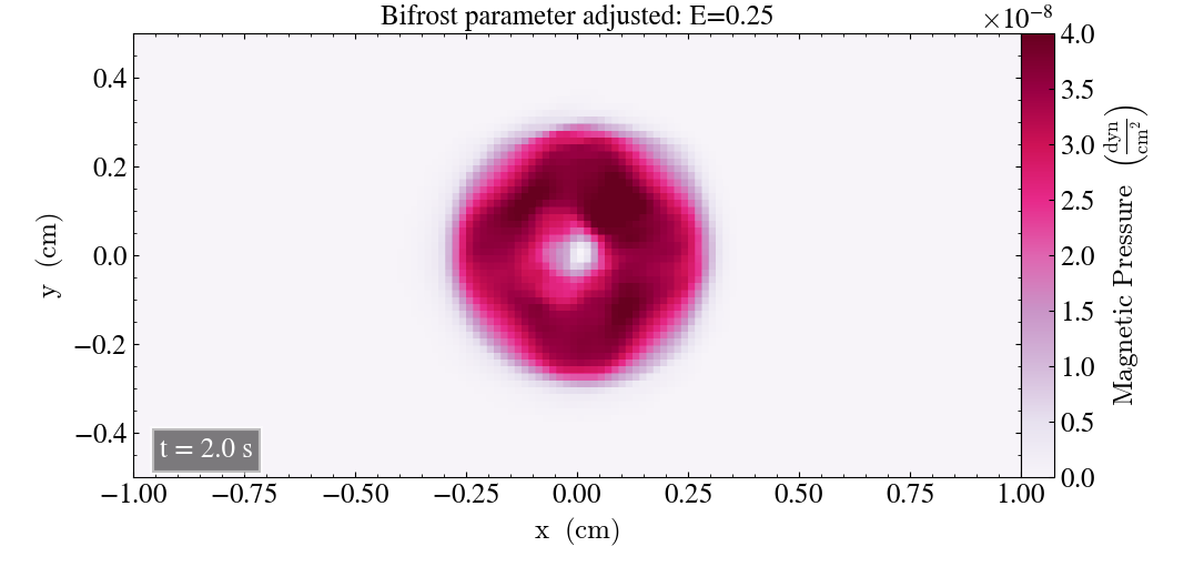
After t=0.2s the above image shows no clear, visible deviations from the initial plot after t=0.2s. After t=2s the pressure is less reduced, and despite a slightly less symmetric hole at the center, the Loop does not seem to have been affected too much by the parameter adjustment.
Below shows the magnetic pressure loop after t=0.2s and t=2s when E is reduced by a factor of 5.


After t=0.2s it’s evident that a factor 5 decrease of E has affected the simulation, as there are ripples within the loop which was not present for the initial simulations. After t=2s there is less reduction of the magnetic pressure, but the loop is visibly deformed, compared to the initial plot.
Below is the magnetic pressure of the Loop for a factor 10 reduction of E after t=0.2s and t=2s.
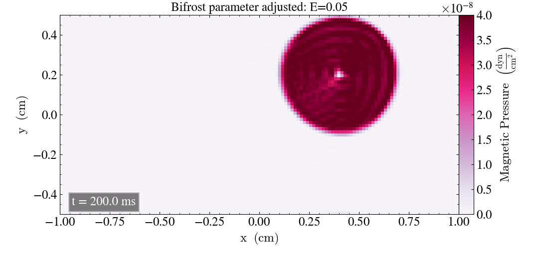
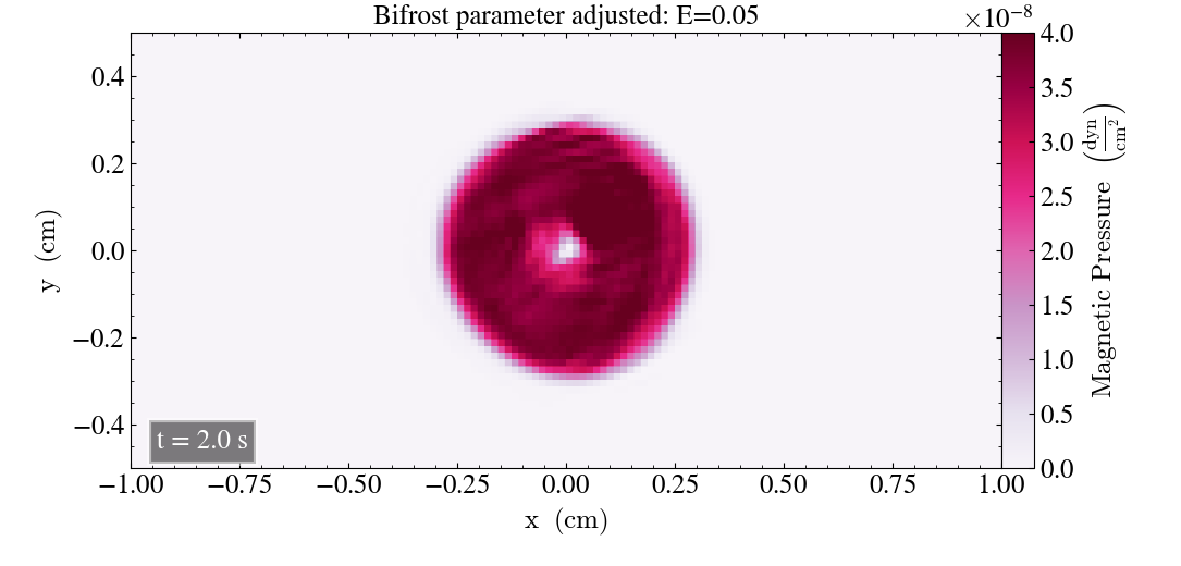
The ripples after t=0.2s above are more prominant with a factor 10 increase of E, as compared to the factor 5 increase. After t=2s there are visible lines in the Loop, demonstrating that it’s not necessarily an optimal result, despite the reduced pressure decline.
Multiple adjustment of bifrost parameters
Now we will study the combined effect, where we adjust multiple bifrost parameters simultaneously. We will report the result of increasing Uv, d & e by a factor of 2. Another adjustment we make is decreasing Ca, U & E by a factor of 2. Finally, we study the effect of increasing Uv, d & e by a factor of 2 while simultaneously decreasing Ca, U & E by a factor of 2. The pressure evolution for these three combinations are plotted below, where the initial result is included for reference. The factor 2 was chosen in order to avoid potential deformation of the Loop, which occured for a factor 5 and 10 reduction of E.
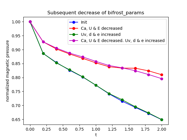
We see that there is little difference between the initial pressure profile and the pressure profile from increasing Uv, d & e by a factor 2, as these lines nearly overlap throughout the simulation. Decreasing Ca, U & E causes less reduction of the pressure in both cases, when Uv, d & e are held fixed and when they’re adjusted as well. The combined decrease and increase seems to give a more steady pressure drop, since we see that the line with reduction only is flattening out before t=1.5s, after which it starts declining at the approximately same rate as the other line after t=1.75s.
The combined adjustments yields a comparable pressure drop compared to the case of N=32 for Miniati & Martin, and with less deformation of the Loop than we had for E=5, which we will show below.
Below, we plot the magnetic pressure of the Loop for the two cases where three bifrost parameters were reduced. We begin with the case where Uv, d & e are held fixed while the remaining parameters are decreased, showing the result after t=0.2s and t=2s in the left and right panel, respectively.
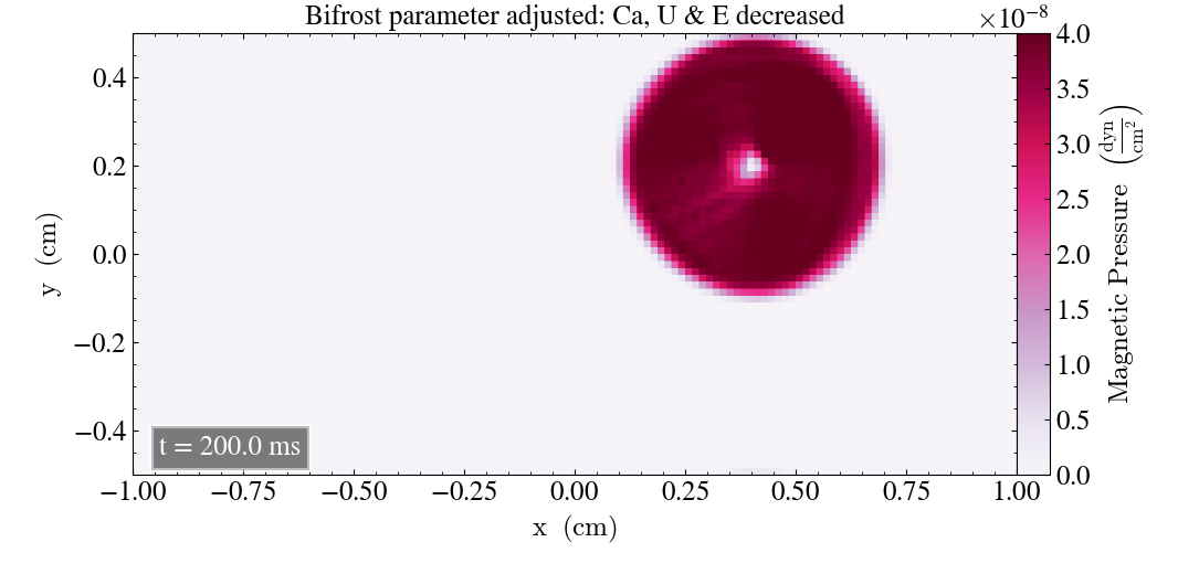
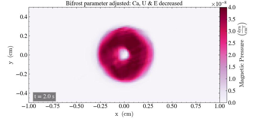
Above, we can see that there are some lines inside the Loop after t=0.2s, which resemble the ones we saw by decreasing E by too much. After t=2s the Loop looks distorted, once again resembling what we saw for the reduction of E.
Below shows the magnetic pressure of the Loop after t=0.2s and t=2s when Ca, U & E are decreased by a factor of 2, while Uv, d & e are increased by a factor of 2.

After t=0.2s there were little noticeable changes when all parameters were adjusted, compared to the plot where we only decreased Ca, U & E. After t=2s there is less deformation of the Loop in the above plot, and the Loop is slightly more circular with less distortion. This effect is not very clear, but the additional increase seems to stabilize the simulation a bit.
Ramses results
For the ramses solver, we plot the behaviour of the Loop, and compare the evolution of the magnetic pressure with the result from the unchanged bifrost result. We will only consider the results in the xy-direction, since the simulation yielded the same results for all three directions.
Initial behaviour
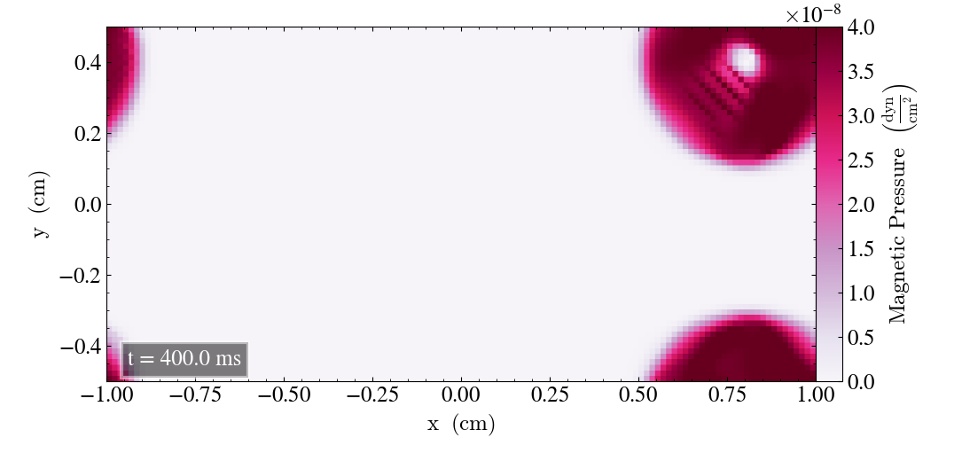
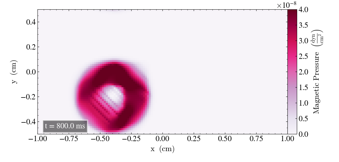
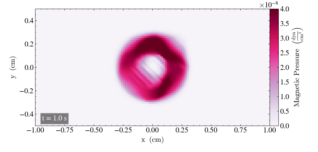
Below are four images showing the initial behaviour of the Loop from t=0s to t=1s. At t=0s the Loop looks fine, but there are visual ripples in the lower left corner appearing as it moves. After t=0.8s (lower left panel), the bottom left of the Loop is very dim and the ripples are still in place. After t=1s, the Loop is dimmer overall and the pressure gap in the Loop’s center has increased its diameter.

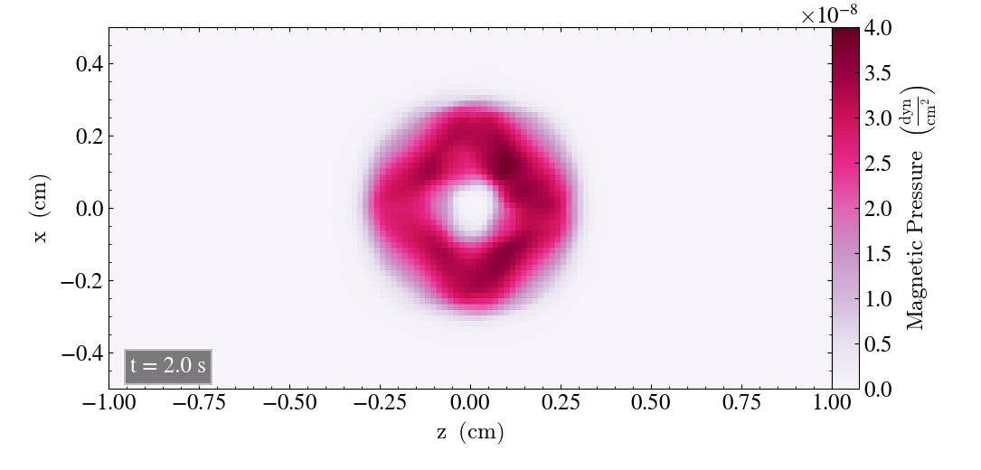
We plot the Loop after t=2s, shown below. The Loop has a dim circular shape, but the main part of it is clearly reduced, and high pressure is noticeable in a more rectangular shape.
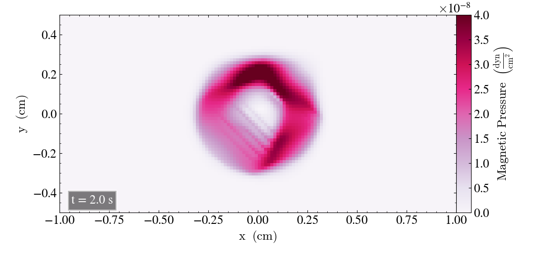
Above we see the Loop after t=2s. It’s clearly deformed, and has a very reduced pressure overall, meaning that the bifrost simulation was far better for this particular experiment and with the particular parameters.
slope_type
When attempting a simulation using slope_type=1, the simulation reached a point where there were multiple infinities and no results were obtained.
Pressure evolution
We now plot the normalized magnetic pressure evolution for the ramses experiment, shown below. The initial pressure evolution of the bifrost solver is also included in order to compare.
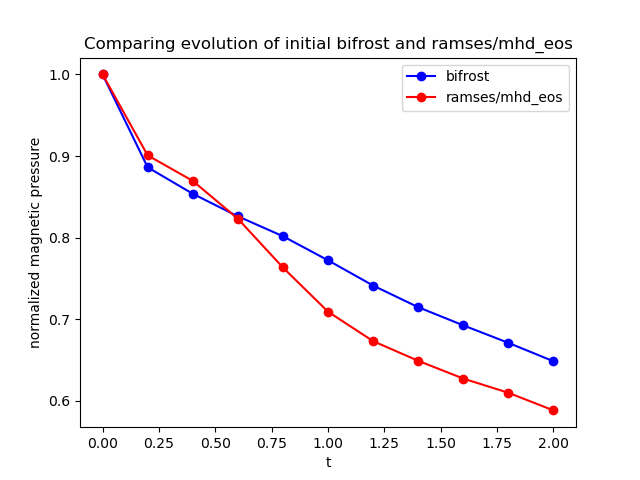
As we can see above, the bifrost solver yields a lower reduction in the magnetic pressure over time. The reduction from the bifrost solver is more steady than the reduction from the ramses/mhd_eos solver, which displays an oscillating behaviour as it declines.
References
Miniati & Martin (2011) - iopscience.iop.org/article/10.1088/0067-0049/195/1/5/pdf
Gardiner & Stone (2005) - arxiv.org/pdf/astro-ph/0501557.pdf